You can run this notebook in ![]() , in
, in ![]() , in
, in ![]() or in
or in  .
.
[1]:
!pip install --quiet climetlab tensorflow
Machine learning example
[2]:
from tensorflow.keras.layers import Input, Dense, Flatten
from tensorflow.keras.models import Sequential
[3]:
import climetlab as cml
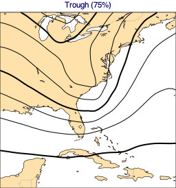
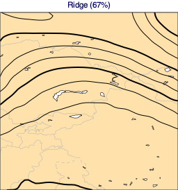
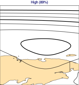
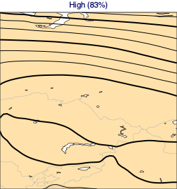
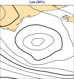
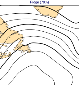
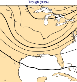
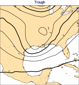
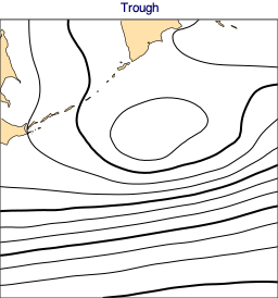
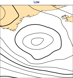
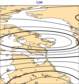
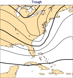
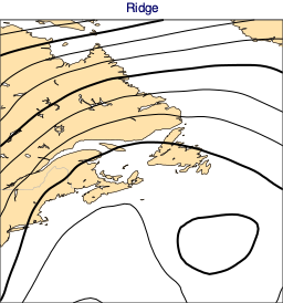
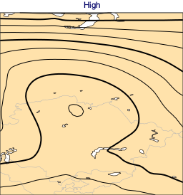
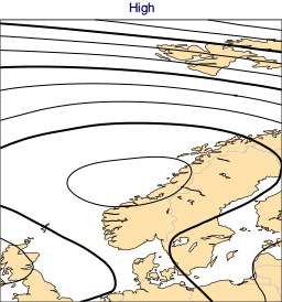
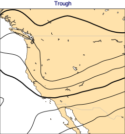
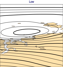
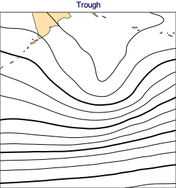
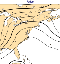
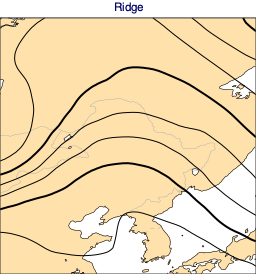
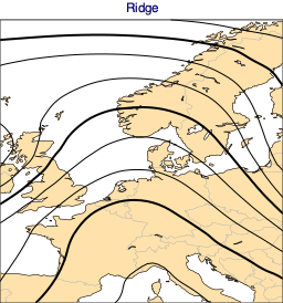
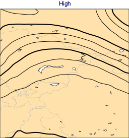
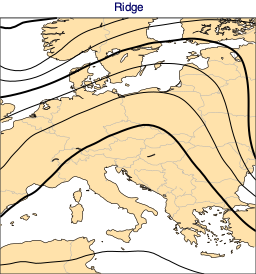
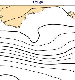
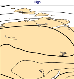
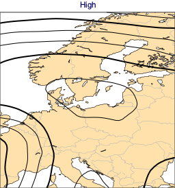
Load the high-low data set and plot all the fields and their label
[4]:
highlow = cml.load_dataset("high-low")
for field, label in highlow.fields():
    cml.plot_map(field, width=256, title=highlow.title(label))


Get the train and test sets
[5]:
(x_train, y_train, f_train), (x_test, y_test, f_test) = highlow.load_data(
    test_size=0.3, fields=True
)
Build the model
[6]:
model = Sequential()
model.add(Input(shape=x_train[0].shape))
model.add(Flatten())
model.add(Dense(64, activation="sigmoid"))
model.add(Dense(4, activation="softmax"))
[7]:
model.compile(optimizer="adam", loss="categorical_crossentropy", metrics=["accuracy"])
print(model.summary())
Model: "sequential"
_________________________________________________________________
Layer (type)                 Output Shape              Param #
=================================================================
flatten (Flatten)            (None, 441)               0
_________________________________________________________________
dense (Dense)                (None, 64)                28288
_________________________________________________________________
dense_1 (Dense)              (None, 4)                 260
=================================================================
Total params: 28,548
Trainable params: 28,548
Non-trainable params: 0
_________________________________________________________________
None
Train the model
[8]:
h = model.fit(x_train, y_train, epochs=100, verbose=0)
Evaluate the model on the test set
[9]:
model.evaluate(x_test, y_test)
1/1 [==============================] - 0s 1ms/step - loss: 0.2691 - accuracy: 0.9167
[9]:
[0.26906612515449524, 0.9166666865348816]
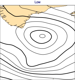
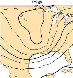
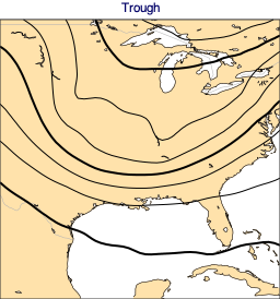
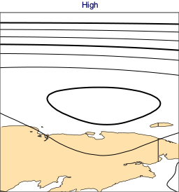
Plot the predictions
[10]:
predicted = model.predict(x_test)

for p, f in zip(predicted, f_test):
    cml.plot_map(f, width=256, title=highlow.title(p))